In the following article, I am going to talk about using Quantum Algorithms to evaluate price Financial Product.
Option Pricing Using Quantum Computers
We will start with most the product Options, which gives power to buyer of option to exercise certain amount of stocks in particular time frame, which helps to reduce the risk of investment professionals.Some commonly used models to value options are Black-Scholes Model, Binomial Option Pricing , and Monte-Carlo Simulation. These theories have wide margins for error due to deriving their values from other assets.
The primary goal of option pricing theory is to calculate the probability that an option will be exercised, or be In-The-Money(ITM), at expiration.
Underlying asset price Stock Price, Exercise Price,Volatility , Interest Rate and time to expiration, which is the number of days between the calculation date and the option’s exercise date, are commonly used variables that are input into mathematical models to derive an option’s theoretical fair value & quite integral in accurately pricing an option.
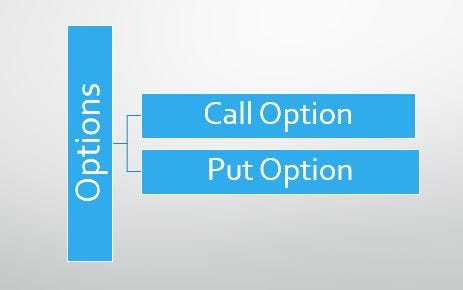 Type of Options
There are two type of options, Call Options , which give control to option holder to buy stocks at fixed amount(strike price) within certain time frame, whereas, Put Options, give control to option holder to sell stocks at fixed amount within certain time frame.
Being the most simplest one, we will go for European Options first, which can be excersied at the time of maturity date only and was modeled and analytically calculated by the Black-Scholes model that assumes stock prices follow a Log Normal Distribution because asset prices cannot be negative.
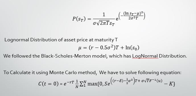 Black Scholes model, Monte Carlo method and Log Normal Distribution
Other assumptions made by the model are that there are no transaction costs or taxes, that the risk-free interest rate is constant for all maturities, that short selling of securities with use of proceeds is permitted, and that there are no arbitrage opportunities without risk.Some of these assumptions do not hold true all of the time.It was also Calculated by Monte Carlo Techniques,
So, as now we have some introduction to a financial derivative lets move on to the Quantum Computing stuff, which will help us to calculate option pricing
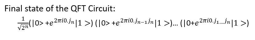
Quantum Fourier Transform
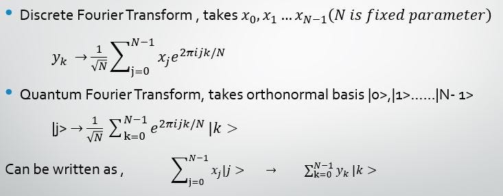 Quantum Fourier Transform, an analogous to Discrete Fourier Transform
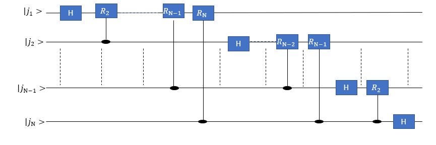 QFT Circuit with end SWAP gate
Phase Estimation Algorithm
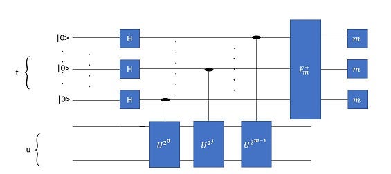 Phase Estimation Circuit
Next we come at phase estimation.
Suppose you have a unitary matrix whose eigenvector is u, and you want to calculate it’s eigenvalue which is form of exp(2*pi*i*phi), where phi is unknown, it helps us to estimate the phi within certain limit.
Phase Estimation, it requires two registers , t and u , where u is eigenvector of some operator with eigenvalue exp(2pi*i*phi), where phi is unkown which we want to estimate,
Assuming we have a black box to prepare the state in u (eigen vector ) and preparing controlled U ^ 2^j for suitable non –ve integer j
T- qubit in state |0> , no. of t qubits determine the no. of digits of accuracy for phi and with what probability we want the phase estimation to be succesull
U qubit contain eigenvector |u> , contains as many qubits as it needs to store |u>
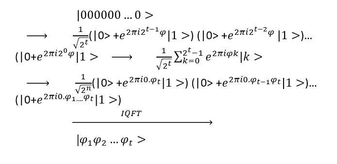 Phase Estimation Calculations
Amplitude Estimation using Phase Estimation
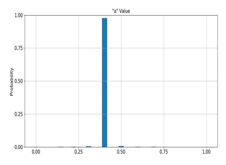
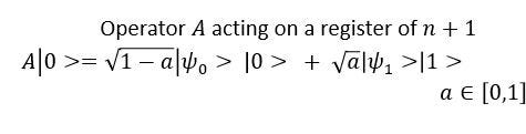 AE is used to estimate “a” in the above equation
Amplitude Estimation, is basically a problem to calculate the probability ,that second qubit in above function is 1 or probability that initial wavefunction yields a particular state. Which is a generalized version of Grovers Search or we can say it is a grover search is special version of Amplitude Estimation, it uses phase estimation and QFT and IQFT.
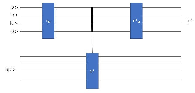 Amplitude Estimation Circuit
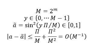 Amplitude Estimation equations
We obtain ⟨f⟩ of random variable X with AE by creating A such that “a”=E[f(x)].
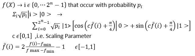
Linearly Controlled Y-rotations
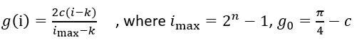
Linearly Controlled Y rotations which helps us to create Piece Wise linear function.Since pay off function for options portfolios is piecewise linear we only need to consider linear functions f:{0,…2^n -1 } → [0,1]
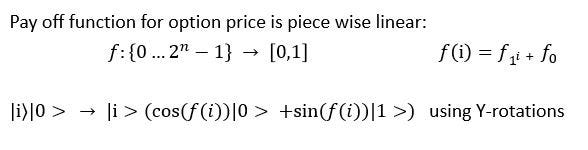
Creating operator that performs equation 2(in above) transforms using controlled Y rotation, with constant term is implemented by rotation of ancilla qubit without any controls and linear term with the control rotation of angle (2^j f1)
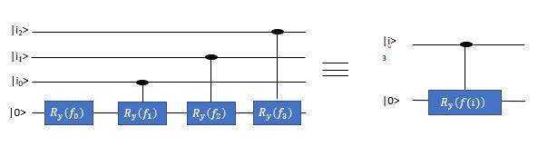 Piece Wise Linear function where 1st gate represent Constant term
Expectation Value using Amplitude Estimation
So, as now we already now the basic and necessary ingredients of Option Pricing and Quantum Computing.
Let’s start with European Style Options which are path independent and can only be exercised at the time of maturity, since it the most simplest options, now a trader will execute it if the strike price is less the asses price at the time of maturity and he will buy (in case of call) and sell(in case of put option) at strike price and than immediately sell (in call) and buy (in put ) in order to make money, the options saves you from the high risk in potentially good deal.
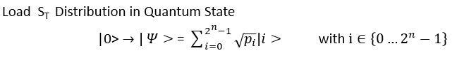
To simulate the option price on quantum computer we will first load the Asset price distribution ‘S’ in quantum state and will truncate it certain size and than discretize this in certain interval.Assuming Black-Scholes assumption we will load Log-normal Distribution.
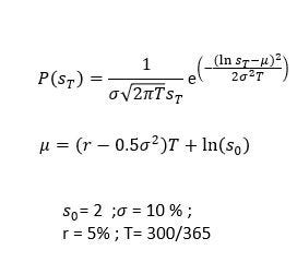 Values of variables to be loaded
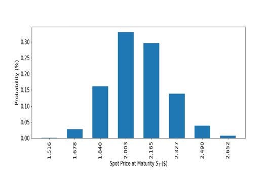 Distribution loaded using 3 qubit
Now, we have to compare the strike price with Spot Price and if the Spot price exceeds strike price we have to change the ancilla bit from initial state of |0> to |1>
 The state after applying comparing circuit, in which can be solved by AE method
In order to use AE, we have to add another ancilla qubit to above qubit , initially in the following state :
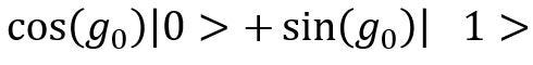
and the final state is mapped to
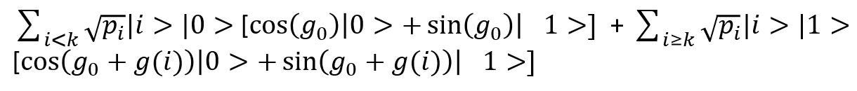
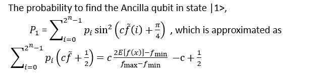
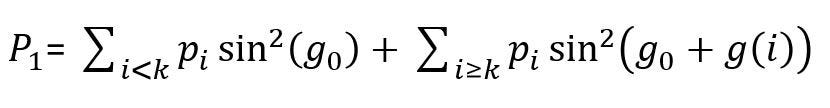
Where we have to calculate the probability that 2nd qubit is in state |1> is given as P
Now, encode Piece Wise Linear Function using earlier Y-rotations .
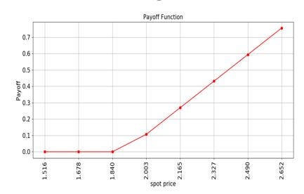
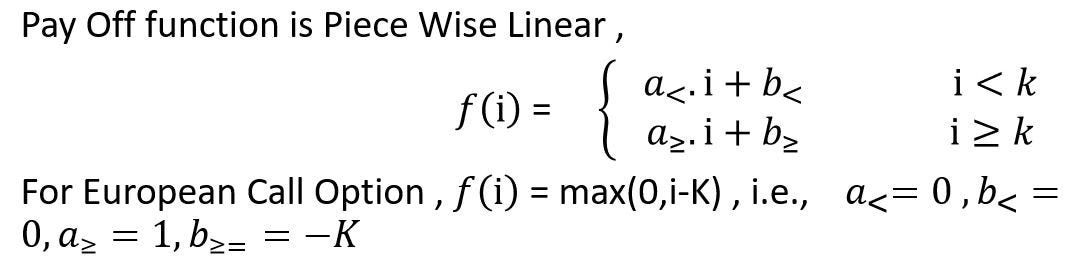 European Function Pay off Function
Final Probability will look like this ,

Pay Off function will look like this:
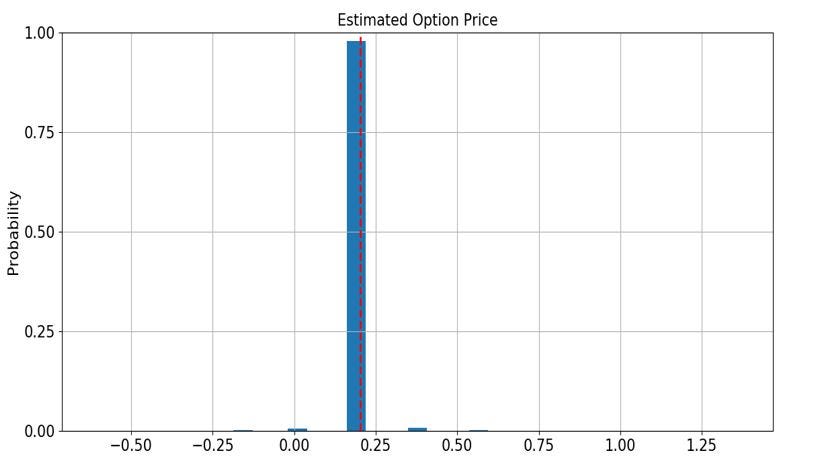
Value of “a” from Amplitude Estimation algorithm will look like following
And the final Option Pricing price will have the following value,where red dashed line shows the analytical value:
References
[1] Option Pricing using Quantum Computers. Daniel J. Egger, Yue Sun, N.Stamatopoulos , C. Zoufal , R.Iten, Ning Shen, Stefan Woerner
[2] Quantuam Risk Analysis. Stefan Woerner , Daniel J. Egger
[3] Quantum Amplitude Amplification and Estimation. Gilles Brassard, Peter Høyer, Michele Mosca , Alan Tapp